How can we measure astronomical distances? One technique is to use "standard candles", which are astronomical objects that have well-known brightnesses. By measuring how bright an object appears to us and knowing the actual brightness from some analysis, we can work out how far the object is from us. We employ the "inverse square law" for light to make this happen and do a bit of math.
 Look for the variable stars. They seem to blink.
Need more on how we use variable stars to measure distance?
If you are new to the idea of variable stars as tools for measuring distances, start with these:
Inverse Square Law
When light leaves the surface of an astronomical object, like a star's photosphere, the resulting light spreads out radially in all directions at the speed of light. All the energy emitted at that same instant can be thought of as being spread out over surface of a sphere. As this imaginary sphere gets bigger, the light gets more spread out. This is why distance matters when looking at a light source. Note the equation for the surface area of a sphere:
\begin{equation*}
A=4\pi{R^2}
\end{equation*}
The closer you are, the more concentrated the light is because the sphere over which it is spread is smaller (smaller radius, R). The farther you get from the source, the bigger the sphere must be when it reaches you (larger radius, R) and consequently, the light is spread out more and so the source seems dimmer.

Illustration of inverse square law.
The physical properties of electromagnetic radiation eminating from a star or other astronomical object is best described using flux which is related to power which is related to energy. Another common way to describe light leaving an astronomical object is through the concept of luminosity. The Stefan-Boltzman relation connections the energy density of a star (how much energy leaves 1 square meter of the star's surfce) and the star's temperature.
\begin{equation*} L=\sigma{T^4}\>[\mathbf{W/m^2}] \end{equation*}We can find the power emitted by the star if we include the entire spherical surface of the star
\begin{equation*} L=\sigma{T^4}(4\pi{R^2})\>[\mathbf{W}] \end{equation*}Don't forget that astronomers can determine the surface temperature of a star using Wien's law. Once the peak wavelength of the light from the star is found, we can get the temperature using the relation:
\begin{equation*} \lambda_{peak}\cdot{T}=constant\>[\mathbf{m\cdot{K}}] \end{equation*}Magnitude vs Luminosity
For historical and convenience reasons, astronomers use a system called magnitude dating back to Hipparcos which uses the star Vega as a reference star. There are many peculiarlities with magnitude. For example a negative magnitude represents a brighter object than does a positive magnitude. Another useful point is that just using light from an image, astronomers can quickly measure the magnitude as seen from earth, the apparent magnitude. That leaves some work to do to get turn the physical brightness or luminosity of the object into the absolute magnitude. The magnitude scale is clunky but still in use - for now.
Globular Clusters
A globular cluster is a very old grouping of stars usually found in the halo or the central region of a galaxy. NGC 3201 is one such globular cluster found in the Milky Way Galaxy. The images used for this activity were taken using the Skynet Robitic Telescope Network run by the University of North Carolina. Yes... they called a robotic telescope system Skynet. The globular cluster was imaged 5 times in a single night by the system. This way, any star that has a periodic change of a day or so will show up in the series of images.
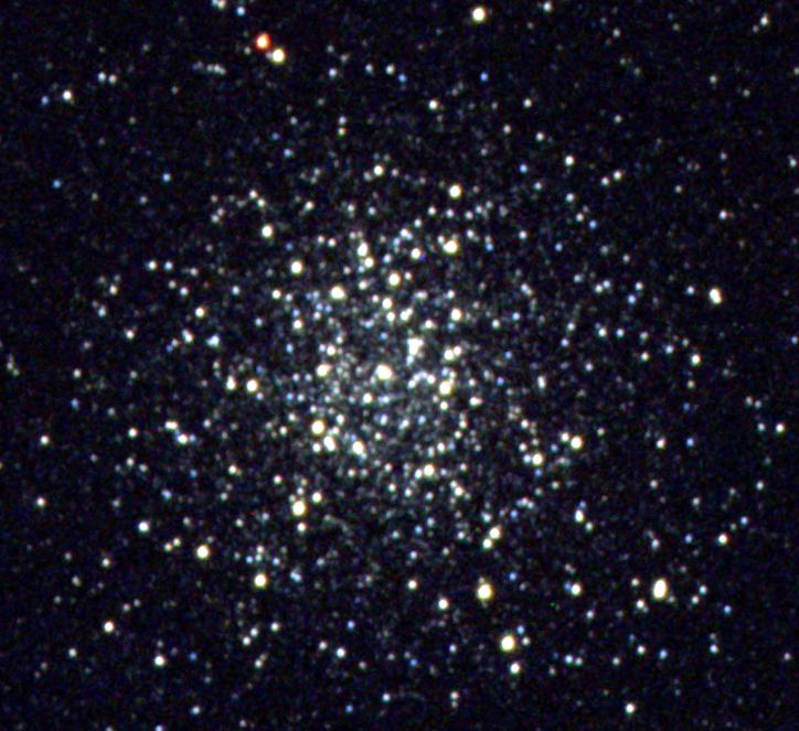 Globular Cluster NGC 3201
For this activity, we are going to study images taken of a variable star in a globular cluster over a single night. This star is known as an RR Lyrae variable star which varies over a period of less than one day. All stars that fall into this class have approximately the same absolute luminosity. That means if all RR Lyrae stars were the same distance from the observer, they would all appear the same brightness.
But stars are, of course, spread out across a galaxy and ours is no exception. So RR Lyrae stars appear to be different brightnesses due to their distances.
Choosing a target
We will study one such star in a globular cluster visible from Earth's southern hemisphere.
In order to determine the magnitude of the star, we will need a known calibration star that is in the field and near the target star. Note that here we have zoomed in a lot on our target star. At this level in this image the only things visible are stars (no galaxies or such) and almost every star visible is a part of the globular cluster.
 Zooming in on the target.
Using the Aladin Sky Atlas, we can overlay data from previous surveys onto the image we took. Note the cirlcles and labels. Some objects have known proper motion values and some are known to be variable stars.
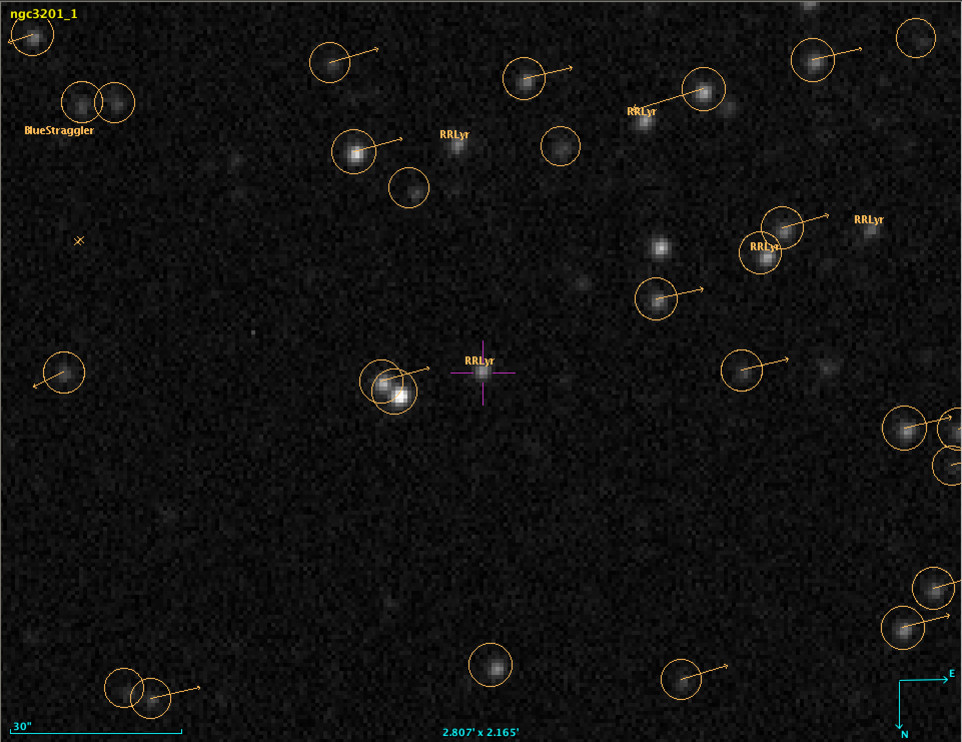 Image loaded into Aladin Sky Atlas with with Simbad source data overlaid.
Note the types of objects seen:
- inCl* - source is a star and part of the cluster.
- BlueStraggler - source is likely result of smaller, redder stars merging
- RGB* - source is a star that has left the main sequence and moved to the red giant branch of the HR diagram
- RRLyr - source is a variable star similar to RR Lyrae with a period less than one day and a known absolute magnitude
- Star - source is a star and not necessarily a member of the cluster
- X - source is an X-ray emitter such as a pulsar (neutron star), or black hole.
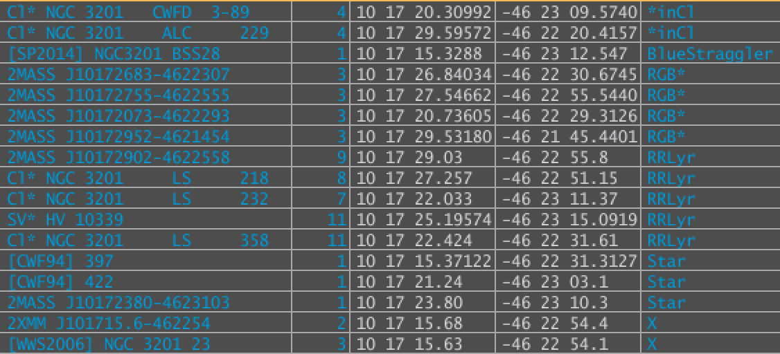 List of targets visible in the field above.
# If you are using Microsoft Azure Notebook, uncomment the line below by removing the #
# We need this line to include the non-standard SEP aperture photometry package.
!pip install --no-deps sep
# Let's import the packages and libraries to help us do our analysis.
# The NumPy package is extremely useful and very common in scientific Python coding.
import numpy as np
# The SEP package is rather specific to our task of performing aperture photometry
import sep
# We import the math package to make our calculations easier to code.
import math
# additional setup for reading the test image and displaying plots
from astropy.utils.data import download_file
from astropy.io import fits

# The MatplotLib package is extremely useful and very common for making plots and displaying images.
import matplotlib.pyplot as plt
from matplotlib import rcParams

# Let's make Jupyter and Matplotlib work together
%matplotlib inline

# This determines the size of the images we display.
rcParams['figure.figsize'] = [8., 8.]
# The known apparent magnitude of calibration star Cl* NGC 3201 CWFD 3-106
# in the visual or green band according to the Simbad database.
# http://simbad.u-strasbg.fr/simbad/sim-id?Ident=Cl*+NGC+3201+CWFD+3-106
m_calibration = 14.81

# The known absolute magnitude of target star Cl* NGC 3201 LS 358
# https://iopscience.iop.org/article/10.1086/344948
M_target = 0.58
# Convenience function for mirroring a image about X and Y
# One of the FITS images was flipped horizontally and vertically and this function helps us fix that.
def mirror_data(data):
    dataout = np.array(data)
    rows = len(data)
    cols = len(data[0])
    for r in range(rows):
        for c in range(cols):
            dataout[rows-1-r][cols-1-c] = data[r][c]
    return dataout
Distance Modulus
If the apparent magnitude and the absolute magnitude of a source are known, once can determine the distance to the source in parsecs using the distance modulus relation. Small m is the apparent magnitude of the source. Big M is the absolute magnitude of the source. The distance is then d. Note the base of the logarithm is 10 in this case. The distance modulus is logarithmic in nature but it is also based on historical uses of magnitudes. Hence a distance modulus of 5 corresponds to a distance of 100 pc. The absolute magnitude scale is based on objects all being located 100 pc away from the viewer. Another example: a magnitude 1 star is exactly 100 times brighter than a magnitude 6 star. \begin{equation*} m - M = -5 + 5\cdot log_{10}(d) \end{equation*}
Coding and Questions
If you need to install Python and Jupyter notebook, the best bet is to install Anaconda.
- Follow the directions and answer the questions listed in the comments of a given block of code.
- Don't be afraid to experiment! This is an interactive lesson using coding. There is always the undo button!
- The code used here is Python 3 which is common for scientific computing. This isn't the only language used in science by any means. It just works well for our purposes here.
- Answer questions directly in the code block using comments. That will be part of your finished product!
- The # means just that line is a comment
- The """ ... """ means everthing between the triple quotes is a comment and can span multiple lines.
- Include your name, the date, and class or period information. Be sure not to leave out any group members!
# Example of a single line comment
"""
    Example of multi-line comment
"""
"""
    Function to find the distance of an astronomical object in parsecs
    if given the apparent, m, and absolute, M, magnitudes of the object.

    Use some algebra and re-arrange the distance modulus equation to return
    the distance in parsecs of the object
    Don't forget how exponents work: x^2 (x squared) would be written as x**2
"""
def distance_modulus(m,M):
    return ...
"""
    Testing the distance modulus: should be approximately 1.0 for the Sun
        m = -26.76 and M =4.81
    There are 648000 arcseconds in 180 degrees of arc. Why do we need that conversion here?
    Is your result close enough to be useful? How can you tell?
    Compare your result with another student.
"""
print(distance_modulus(-26.76,4.81)*648000/math.pi)
"""
    Function to find the apparent magnitude of an object if given the
    flux (or counts) found via aperture photometry.
    http://classic.sdss.org/dr7/algorithms/fluxcal.html
    This function depends on the filters used and the mininum about of
    flux the filter allows. Likely you shouldn't change anything here.
"""
def app_mag(flux):
    return -2.5*math.log10(flux/(25.11*10**8))
"""
    Testing the apparent magnitude function:
    should be 14.81 for our calibration star according to literature.
    https://iopscience.iop.org/article/10.1086/344948
"""
print(app_mag(2967.8))
"""
    This functions consumes as input the filename as a string and a "flag"
    for whether or not this image should be mirrored. To mirror an image
    is to flip the image in both the horizontal and vertical direction.

    The data is returned as a 2-D NumPy array. This array represents the
    light received by each pixel in the camera.

"""
def get_image_data(filename, mirror=False):
    # process filename as FITS file
    file = filename
    image_file = download_file(file, cache=True )

    data = fits.getdata(image_file)

    if mirror==True:
        data = mirror_data(data)

    # We need this line to allow the SEP package to work with our
    # AstroPy formatted FITS file
    # See: https://sep.readthedocs.io/en/v1.0.x/tutorial.html#Finally-a-brief-word-on-byte-order
    data = data.byteswap().newbyteorder()

    return data
"""
    This functions consumes as input a 2D NumPy array from a FITS image.
    The data returned is the data with the background subtracted and also
    background data to use in other functions.

    Removing the background improves the signal to noise ratio so our sources
    can be extracted more easily.
"""
def subtract_background(data):
      # measure a spatially varying background on the image
    bkg = sep.Background(data)

    # evaluate background as 2-d array, same size as original image
    bkg_image = bkg.back()
    # bkg_image = np.array(bkg) # equivalent to above

    # evaluate the background noise as 2-d array, same size as original image
    bkg_rms = bkg.rms()
    data_sub = data - bkg

    return data_sub, bkg
Why subtract the background?
If we have an astronomical image, the things we care about, like stars, might be hidden in the excess light and noise of our image. By using the SEP package to find and remove the background, we improve the signal to noise ratio. We want more signal and less noise. Finding ways to improve the S/N is a very common practice is scientific analysis. The 1st image has the background, the 2nd shows the background and the 3rd image is missing the background.
data = get_image_data('http://jimmynewland.com/astronomy/ngc-3201/ngc3201_1.fits')
data_sub, bkg = subtract_background(data)
bkg_image = bkg.back()
m1, s1 = np.mean(data), np.std(data)
plt.imshow(data, interpolation='nearest', cmap='gray',vmin=m1-s1, vmax=m1+s1, origin='lower')
# show the background
plt.imshow(bkg_image, interpolation='nearest', cmap='gray', origin='lower')
m2, s2 = np.mean(data_sub), np.std(data_sub)
plt.imshow(data_sub, interpolation='nearest', cmap='gray',vmin=m2-s2, vmax=m2+s2, origin='lower')
"""
    This function consumes the subtracted data, the background, and
    the x and y coordinates for the subsection of the image containing the target star.
    There are 2 XY pairs for the "bounding box" we want within the original image.
    We then plot ellipses around each detected source and finally return the list
    of sources extracted.
"""
def extract_sources(data_sub, bkg, x1, y1, x2, y2):
    # perform the extraction
    objects = sep.extract(data_sub, 1.5, err=bkg.globalrms)

    # display the image
    from matplotlib.patches import Ellipse

    # plot background-subtracted image
    fig, ax = plt.subplots()
    m, s = np.mean(data_sub), np.std(data_sub)
    im = ax.imshow(data_sub, interpolation='nearest', cmap='gray',
               vmin=m-s, vmax=m+s, origin='lower')
    plt.xlim(x1,x2)
    plt.ylim(y1,y2)

    # plot an ellipse for each object
    for i in range(len(objects)):
        e = Ellipse(xy=(objects['x'][i], objects['y'][i]),
                width=6*objects['a'][i],
                height=6*objects['b'][i],
                angle=objects['theta'][i] * 180. / np.pi)
        e.set_facecolor('none')
        e.set_edgecolor('red')
        ax.add_artist(e)
    plt.show()

    return objects
"""
    This function helps us chose the center of the given region
    so we can find the target closest to the center.

    We consume the 2 XY pairs and return the ordered pair for the
    center of the image as a tuple.
"""
def select_target(x1, y1, x2, y2):
    # select our target star by x and y position in the image
    cen_x = x1 + (x2-x1)/2
    cen_y = y1 + (y2-y1)/2

    return cen_x, cen_y
"""
    This function consumes our list of extracted targets along with
    the data after subtraction, the background, and the center x and
    center y values.

    We then go through the list and find the flux for the target closest
    to the center (within 5).

    The flux for the target star is then returned.
"""
def get_target_flux(objects, data_sub, bkg, cen_x, cen_y):
    target_flux = 0

    for i in range(len(objects)):
        curr_x = objects[i]['x']
        curr_y = objects[i]['y']

        # Get the flux for target star (center)
        if curr_x > cen_x-5 and curr_x < cen_x+5 and curr_y > cen_y-5 and curr_y < cen_y+5:
            # find the flux of object nearest the center
            flux, fluxerr, flag = sep.sum_circle(data_sub, objects[i]['x'], objects[i]['y'],
                                     3.0, err=bkg.globalrms, gain=1.0)
            target_flux = round(int(flux))
    return target_flux
"""
    This function consumes our list of extracted targets along with
    the data after subtraction, the background, and the center x and
    center y values.

    We then go through the list and find the flux for the calibration star.
    Note: this will work ONLY for these images. Changing the calibration star
    would require a tedious by-hand analysis to locate the new position.

    The flux for the calibration star is returned.
"""
def get_calib_flux(objects, data_sub, bkg, cen_x, cen_y):
    for i in range(len(objects)):
        curr_x = objects[i]['x']
        curr_y = objects[i]['y']

        # Get flux of calibration star (below)
        if curr_x > cen_x-5 and curr_x < cen_x+5 and curr_y > cen_y-81-15 and curr_y < cen_y-81+15:
            # find the flux of object nearest the center
            flux, fluxerr, flag = sep.sum_circle(data_sub, objects[i]['x'], objects[i]['y'],
                                     3.0, err=bkg.globalrms, gain=1.0)
            calibration_flux = round(int(flux))
    return calibration_flux
"""
    This functions consumes:
        a filename which can be local or a URL for a FITS file,
        the starting and ending points marking the bounding box for the image,
        and whether or not the image needs to be flipped (both vertical and horizontal)
    This function returns:
        the apparent magnitude of the target star
    The process image function is where we bring the steps together.
    1) Get the image data using the filename and mirror flag.
    2) Get the subtracted data and background using the data from step 1
    3) Extract a list of sources using the subtracted data, the background
        and the given x and y pairs (2 x values and 2 y values).
    4) Set the target as the center of the image.
    5) Get the flux for our target star.
    6) Get the flux for out calibration star.
    7) Determine the apparent magnitude of the calibration star.
    8) Calibrate the apparent magnitude of the target star.
    9) Print and return our target star magnitude.
"""
def process_image(filename, x1=0, y1=0, x2=2048, y2=2048, mirror=False):
    # Get image data
    data = ...

    # Measure and subtract background
    data_sub, bkg = ...

    # Extract sources
    objects = ...

    # Select target (center)
    cen_x, cen_y = ...

    # Find target star flux
    target_flux = ...

    # Find the calibration star flux
    calibration_flux = ...

    # Convert the flux into an apparent magnitude
    m_cal_ap = ...

    # Calibrate the magnitudes for the target and calibration star
    f_cal = m_cal_ap/m_calibration # Calibration factor
    m_cal = m_cal_ap/f_cal

    # Convert the flux into an apparent magnitude
    m_tar_ap = ...

    # Calibrate the magnitude of the target
    m_tar = m_tar_ap/f_cal

    print("App. mag of target star m = : "+str(m_tar))
    print("App. mag of calib. star m = : "+str(m_cal))

    # Return the magnitude for the distance calculation
    return m_tar
# Empty list meant to hold calculated magnitudes for target star returned from process_image function
target_mags = []
"""
    Run process_image using the following parameters:
    filename='http://jimmynewland.com/astronomy/ngc-3201/ngc3201_1.fits'
    x1=860
    x2=1060
    y1=668
    y2=868
"""
m_out = process_image(..., ..., ..., ..., ...)
target_mags.append(m_out)
"""
    Run process_image using the following parameters:
    filename='http://jimmynewland.com/astronomy/ngc-3201/ngc3201_2.fits'
    x1=869
    x2=1069
    y1=673
    y2=873
"""
m_out = process_image(..., ..., ..., ..., ...)
target_mags.append(m_out)
"""
    Run process_image using the following parameters:
    filename='http://jimmynewland.com/astronomy/ngc-3201/ngc3201_3.fits'
    x1=205
    x2=435
    y1=190
    y2=420
"""
m_out = process_image(..., ..., ..., ..., ...)
target_mags.append(m_out)
"""
    Run process_image using the following parameters:
    filename='http://jimmynewland.com/astronomy/ngc-3201/ngc3201_4.fits'
    x1=262
    x2=462
    y1=195
    y2=395
"""
m_out = process_image(..., ..., ..., ..., ...)
target_mags.append(m_out)
"""
NOTE: This image was taken by a different telescope in the network
and subsequently was slightly different than the other 4 images.
Be sure to set mirror to True for this star.
    Run process_image using the following parameters:
    filename='http://jimmynewland.com/astronomy/ngc-3201/ngc3201_5.fits'
    x1=641
    x2=841
    y1=709
    y2=909
    mirror=True
"""
m_out = process_image(..., ..., ..., ..., ..., ...)
target_mags.append(m_out)
# Print out the list of determined magnitudes for target star from the 5 images.
# Note the more negative a magnitude is, the brighter.
# Did the star vary in brightness over the 5 images as we expect for an RR Lyrae?
# Do the magnitudes make sense? Are any way brighter or dimmer than the others?
print(target_mags)
# Students see
# print(...)
# You should select the brightest magnitude to use in the distance modulus calculation

# The command np.min(list) will return the smallest value in list.
# Why would we want the smallest magnitude if we want the brightest one from the list?
brightest = np.min(target_mags)
# Students see
# brightest = ...

# Subtract off the reddening factor from our brightest value: 0.25
# The 0.25 is to correct for dust scattering some of the light.
# This is known as stellar reddening. The value was taken from literature.
m_target = brightest-0.25
# Students see
# m_target = ...

# Print our new apparent magnitude for our target star.
# Students see
# print(...)
print(m_target)
How far away is NGC 3201?
According to other researchers, the distance to NGC 3201 is 16 kly or 4.9 kpc. How does our analysis compare?
# Finally we find the distance to the globular cluster based on our analysis.
# Convert the given distance from pc to kpc.
distance = distance_modulus(m_target,M_target)/1000

# Print the distance in kpc .
print('Distance to NGC 3201: '+str(...)+' kpc')
Wrap up
Be sure to submit your final work! From within Jupyter notebook, you can select
- File->Download as-> html (.html) and you'll get a single HTML file you can submit as your finished product. Be sure to keep a copy of the final output just in case you need to submit it again. If you want the Jupyter notebook in an editable form, select
- File->Download as-> Notebook (.ipynb) and you'll get a single Jupyter notebook file.
You will need Python and Jupyter notebook on whatever computer you want to use to edit the notebook file. You can also use Microsoft Azure Notebooks on the web.
References
- Much of the photometry code comes from Python library for Source Extraction and Photometry
- The FITS file handling comes from python4Astronomers
- Be sure to check out my originalobservational project For more information, contact Jimmy Newland

This work is licensed under a Creative Commons Attribution-NonCommercial-ShareAlike 4.0 International License.